Hybrid-DenseViTGRU-XAI-Voice

Hybrid DenseNet–ViT–GRU With XAI for Mental Stability Detection From Voice Data

This repository contains the implementation of a hybrid DenseNet–Vision Transformer (ViT)–GRU model with Explainable AI (XAI) for diagnosing psychological stability using voice data. The pipeline converts raw audio into log-mel spectrograms, trains a hybrid deep model with SMOTE + augmentation, and explains predictions using Grad-CAM, LIME, and SHAP.

---

📄 Research Paper

Title: Hybrid Deep Models for Mental Health Detection with XAI Techniques (DenseNet–ViT–GRU)
Authors: Rafiul Islam, Dr. Md. Taimur Ahad, et al.
Status: Ongoing Research / Manuscript in Preparation
Note: The final paper link will be added here after submission/acceptance.

---

📊 Project Overview

Mental health diagnostics are often subjective and dependent on self-reports and clinician observation. This research proposes a voice-based diagnostic approach using a hybrid deep learning architecture that combines:

• DenseNet-style CNN for extracting local time–frequency patterns
• Vision Transformer (ViT) for capturing long-range dependencies
• GRU for sequential aggregation of learned representations
• XAI methods to interpret predictions and increase transparency

Key Highlights:

• Feature Extraction: Log-mel spectrograms generated from audio signals.
• Model Architecture: DenseNet (local) → ViT (global context) → GRU (sequence learning).
• Class Balancing: SMOTE applied on training spectrogram features (train-only).
• Augmentation: SpecAugment-style time/frequency masking + random time/frequency shifts.
• Evaluation: 5-Fold Cross Validation with stable ROC-AUC across folds.
• Explainability: Grad-CAM heatmaps + LIME & SHAP explanations on spectrograms.
• Ethics: Dataset is not included in this repo due to privacy/ethical constraints.

---

📋 Requirements

• Python 3.8 or above
• TensorFlow / Keras
• Librosa
• NumPy, Pandas, Matplotlib, Scikit-learn
• Imbalanced-learn (SMOTE)
• OpenCV, scikit-image
• LIME, SHAP

---

🛠 How to Run

1. Install Dependencies:

   pip install librosa matplotlib numpy pandas seaborn tensorflow keras scikit-learn tqdm imbalanced-learn opencv-python scikit-image lime shap
   

2. Prepare Dataset: Create the following folder structure:

   data/
   ├── mentally_stable/
   │   ├── *.wav
   └── mentally_unstable/
    ├── *.wav
   

Recommended audio settings (from experiments):

• Sample Rate: 48,000 Hz
• Segment Length: 2 seconds
• Spectrogram: log-mel (128 mel bands)

⚠️ Dataset is not included in this repository due to privacy/ethical constraints.

1. Run Notebook: Open and execute:
   • notebooks/Final_Result_Dense_ViT_GRU_With_XAI.ipynb

---

📊 Results

✅ Data & Preprocessing Visuals

• Waveform examples (Stable vs Unstable)
  

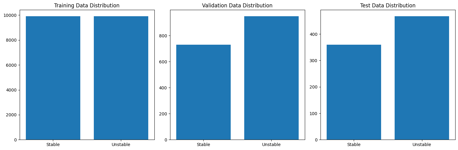
• Train/Validation/Test distribution
  

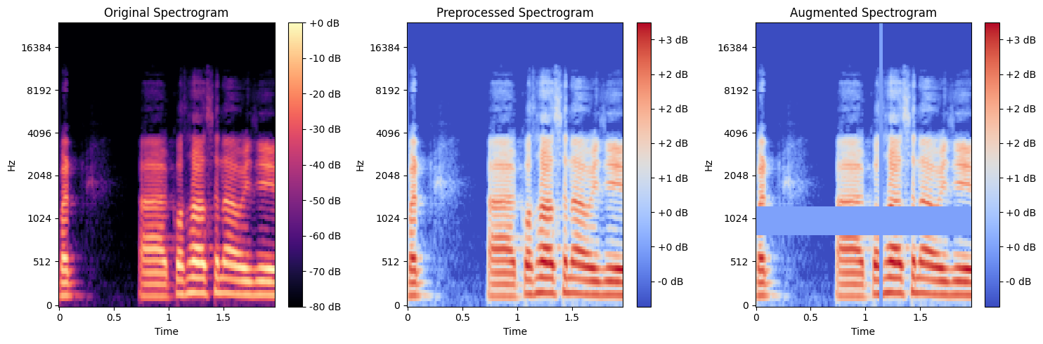
• Spectrogram pipeline: Original → Preprocessed → Augmented
  

---

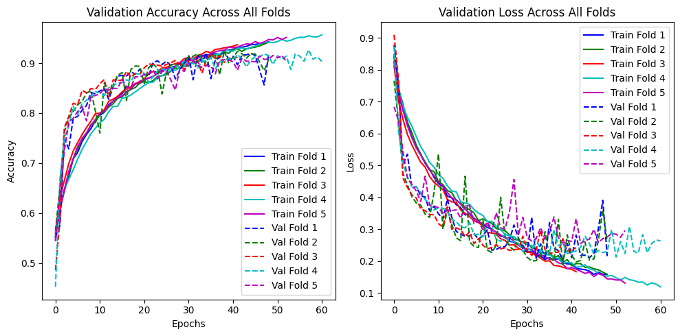
✅ 5-Fold Cross Validation Training Behavior

• Validation accuracy and loss across folds
  

---

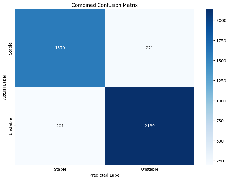
✅ Confusion Matrix (Combined Across All Folds)

The combined confusion matrix across folds shows strong separation between classes:

• Stable → Stable: 1579
• Stable → Unstable: 221
• Unstable → Stable: 201
• Unstable → Unstable: 2139

This yields an overall combined accuracy of ~89.81%.

---

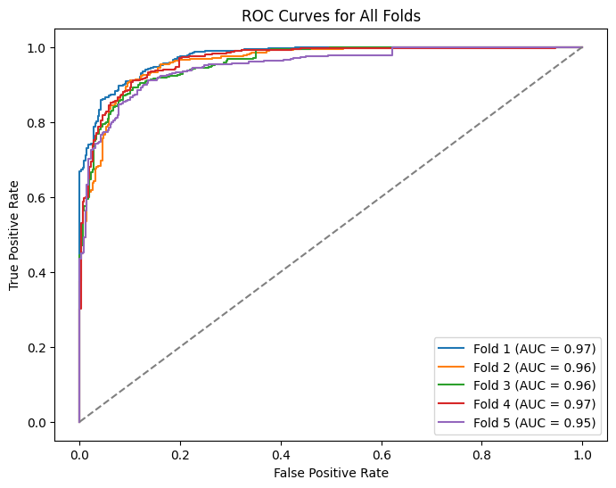
✅ ROC Curves (All Folds)

AUC per fold:

• Fold 1: 0.97
• Fold 2: 0.96
• Fold 3: 0.96
• Fold 4: 0.97
• Fold 5: 0.95

Mean AUC ≈ 0.962.

---

🔍 Explainable AI (XAI) Results

This project includes three explanation techniques to interpret model decisions on spectrogram inputs.

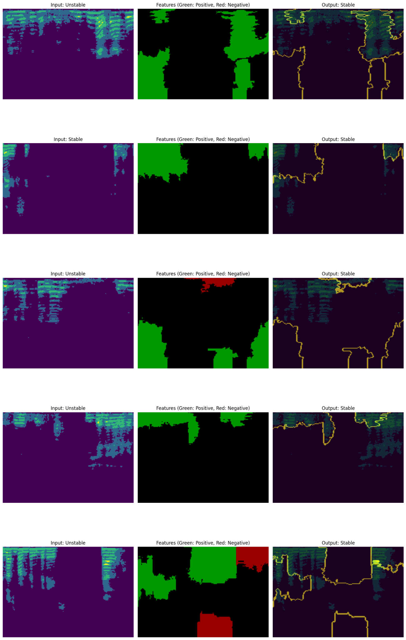
1) LIME (Local Explanations)

LIME highlights positive (green) and negative (red) contributing regions for individual predictions.

---

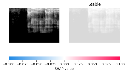
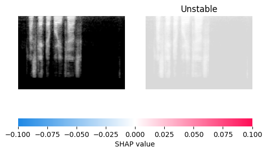
2) SHAP (Global + Local Explanations)

SHAP visualizes contribution strength using Shapley-value inspired attribution.

• Stable sample (SHAP explanation)
  

• Unstable sample (SHAP explanation)
  

---

3) Grad-CAM (Model Attention Heatmap)

Grad-CAM highlights the most influential time–frequency regions used by the model.

---

📜 Citation

If you use this work, please cite this repository (until the paper is published):

• Islam, R., Ahad, M. T., et al. (2026). Hybrid DenseNet–ViT–GRU With Explainable AI for Voice-Based Psychological Stability Detection. GitHub Repository.

(Replace this with the final paper citation after publication.)

---

🧑‍💻 Author

• Rafiul Islam

• Researcher

  Machine Learning & AI Engineer

• Daffodil International University (CSE)
• Junior Machine Learning Engineer @ Bondstein Technologies Ltd.

---

⚠️ Disclaimer

This project is for research and educational use only and does not provide medical advice or clinical diagnosis. Always consult qualified professionals for mental health concerns.